Data access
OCTOPUS data can be viewed and exported through a bespoke Web interface or accessed directly via Web Feature Service (WFS). The latter allows users to access database content via third party software such as Geographic Information Systems (GIS), or R language. OCTOPUS data is served by GeoServer 1, an open server solution for sharing geospatial data. Unless data from OCTOPUS is explicitly downloaded and locally stored by the user, it will remain cloud-borne, so the user will not have to care about data storage and being up-to-date.
Web Feature Service
This user guide and brief demonstration of capabilities outlines how to use WFS through third-party software, specifically QGIS and/or R software environment as these software solutions are free, open-source and highly versatile.
WFS in a nutshell
GetCapabilities, DescribeFeatureType, and GetFeature. Calling GetCapabilities will generate a standardised, human readable meta-dataset that describes a WFS service and its functionality. DescribeFeatureType produces an overview of supported feature types, and GetFeature fetches features including their geometry and attribute values, i.e, variable fields.WFS data access via QGIS
After opening QGIS, start a new project: Project > New
In the Browser pane, select WFS/OGC API Features > New Connection…
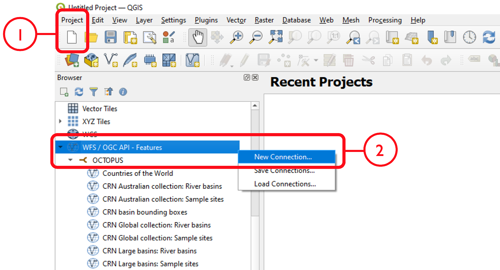
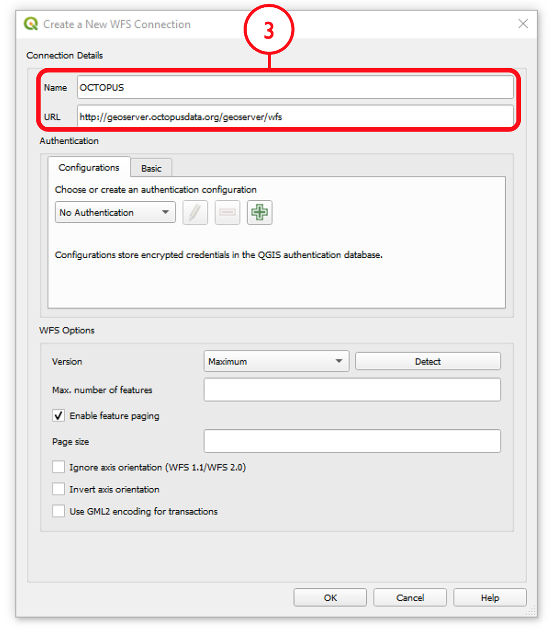
Name the new connection (e.g., ‘OCTOPUS’) and insert the link http://geoserver.octopusdata.org/geoserver/wfs in the URL field. Click OK. All available OCTOPUS collections will appear in the Browser pane once a connection is established
To add a collection of interest, right click on that collection in the Browser pane and select Add Layer to Project. The collection will appear in the Layers pane. Alternatively, click + drag the layer of interest into the Layers pane
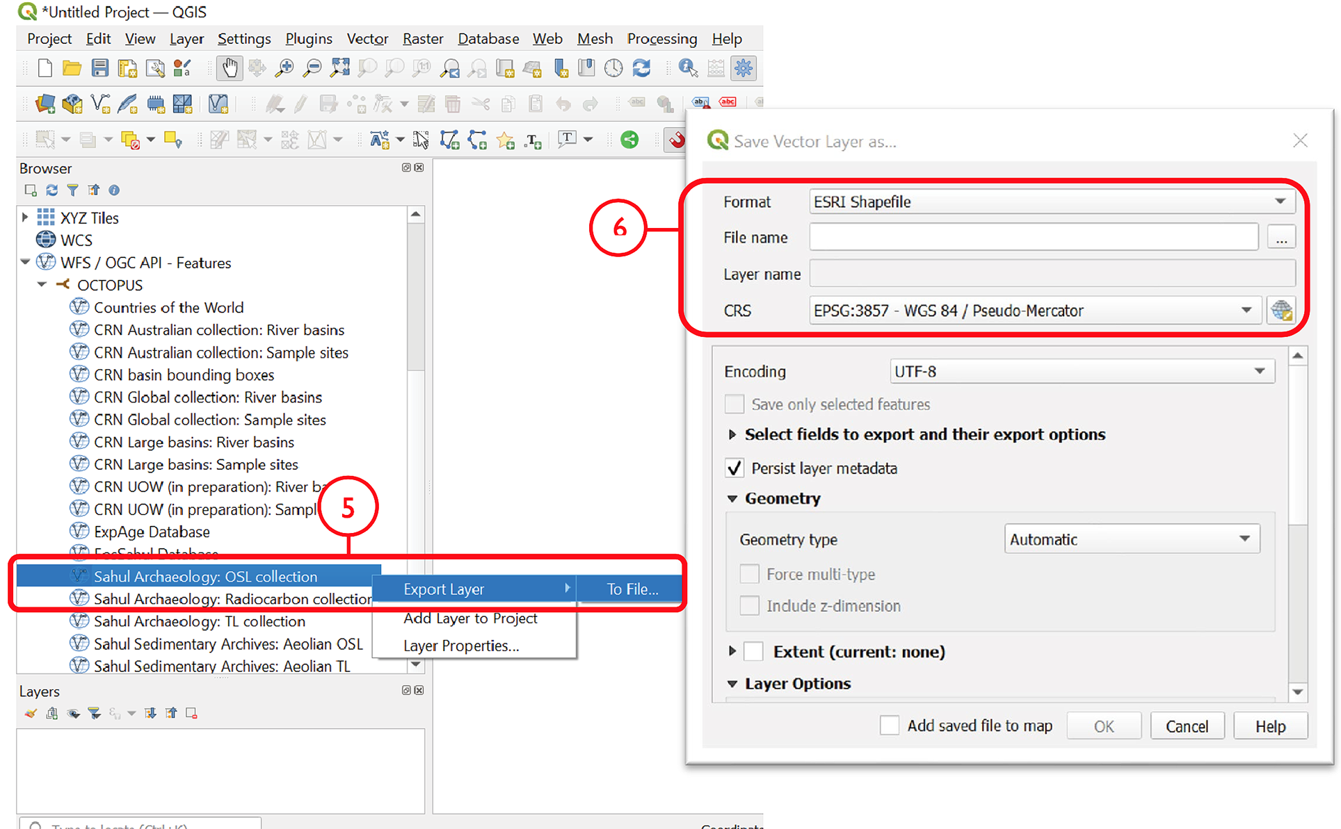
To locally store a collection, select Export Layer > To File
Select a file format and specify a file name and save location via the ‘…’ button. Select the coordinate reference system (CRS) of choice; OCTOPUS v.2 collections use EPSG: 3857 (WGS84 Pseudo-Mercator)
To add a saved shapefile to the project, navigate to the main menu > Layer > Add Layer > Add Vector Layer. Selecting the .shp, .dbf or .shx file (of the six separate files that constitute the shapefile) will open the collection in the Layers pane
Excursus. Obtaining obfuscated geographical coordinates in QGIS
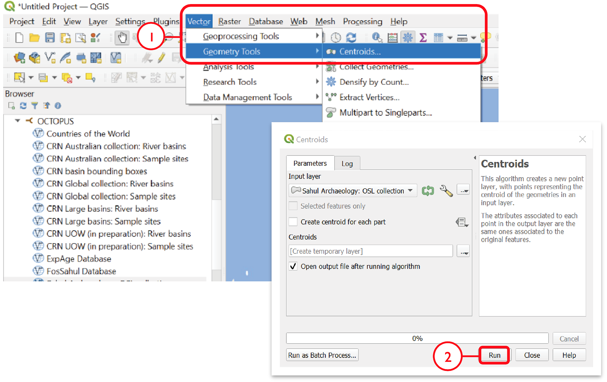
Sites belonging to OCTOPUS data collections SahulArch and FosSahul are potentially culturally sensitive. As a result, coordinates have been obfuscated for these collections using a 25-km radius randomising algorithm. These former point data are represented by polygons now and coordinates are not pushed with the attribute table, or the .csv file if the collection is exported. Follow these steps to obtain obfuscated coordinates (keeping in mind the uncertainty introduced by obfuscation) for these collections by calculating polygon centroid points:
Navigate to the main menu > Vector > Geometry Tools > Centroids…
Select the collection of interest as the Input Layer, and click Run
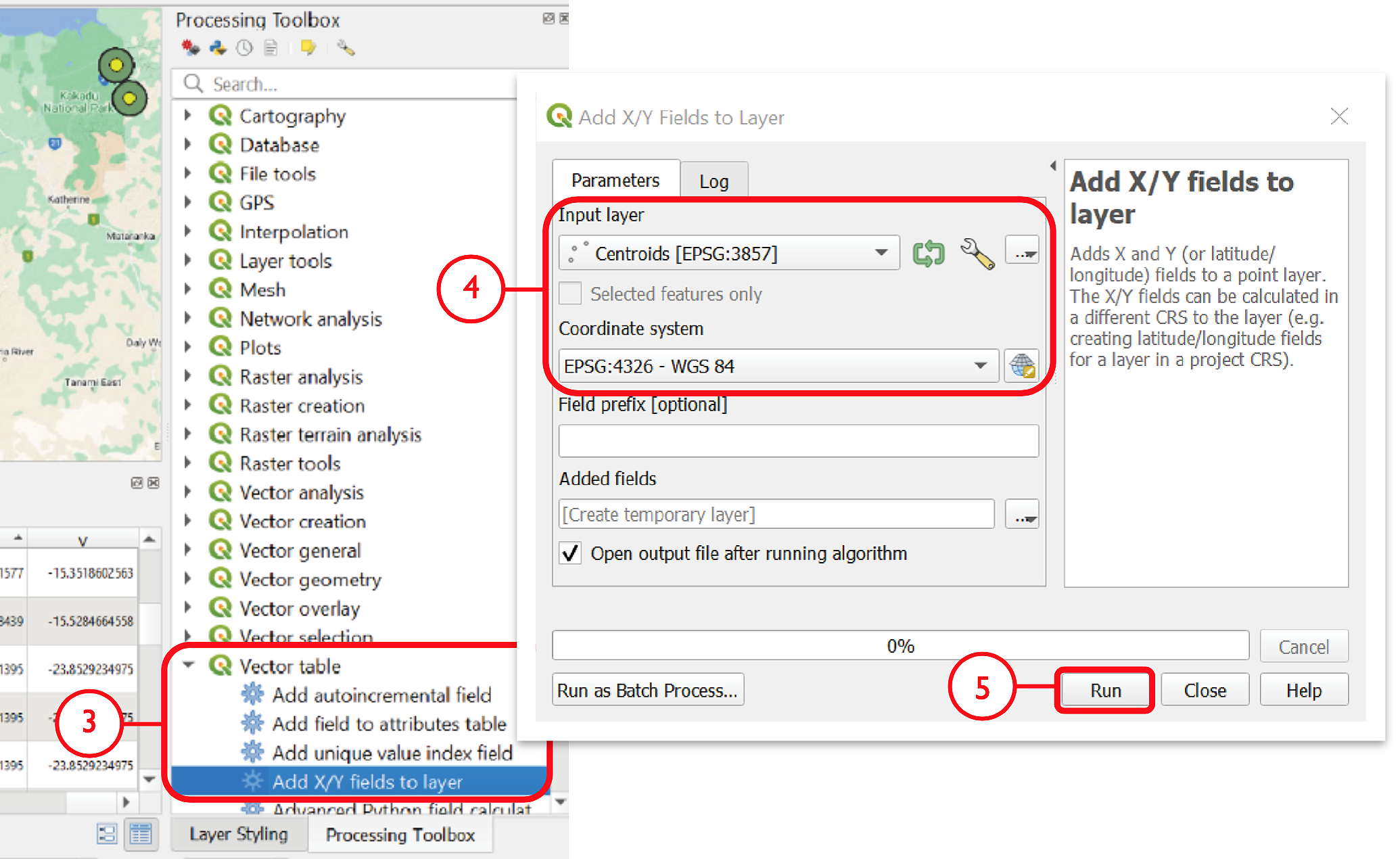
To save coordinates, go to the Processing Toolbox pane and select Vector table > Add X/Y fields to layer
Input Layer should appear as the generated centroids, and the coordinate system must be kept as default EPSG: 4326 – WGS84
Click Run. This will generate a new layer, Added Fields, in the Layers pane. In the Attribute Table, fields for ‘x’ (longitude) and ‘y’ (latitude) will appear at the end of the table with corresponding coordinates for each point feature
WFS data access via R/RStudio
The below demo R script fetches, via WFS, spatial layers including rich attribute data from OCTOPUS database and generates a scatter plot and an interactive map representation, respectively.
Important
The script requires the below packages. If not installed on your machine yet, run
install.packages(c("sf","httr","tidyverse","ows4R","viridis", "mapview", dependencies = TRUE))
and you’ll be all set up.
First we’re going to load the required packages
library(sf) # Simple features support (sf = standardized way to encode spatial vector data)
library(httr) # Generic web-service package for working with HTTP
library(tidyverse) # Workhorse collection of R packages for data sciences
library(ows4R) # Interface for OGC web-services incl. WFS
library(viridis) # Predefined colorblind-friendly color scales for R
OK, we’re ready to go now. In the following we store the OCTOPUS WFS URL in an object. Then, using the latter, we establish a connection to OCTOPUS database.
OCTOPUSdata <- "http://geoserver.octopusdata.org/geoserver/wfs" # store url in object
OCTOPUSdata_client <- WFSClient$new(OCTOPUSdata, serviceVersion = "2.0.0") # connection to db
Let’s see what is there, i.e. show all available layer names and titles
OCTOPUSdata_client$getFeatureTypes(pretty = TRUE) # show available layers and titles
The above WFS request should yield the following overview
                                           name                                      title
1                    be10-denude:crn_aus_basins    CRN Australian collection: River basins
2                   be10-denude:crn_aus_outlets    CRN Australian collection: Sample sites
3                    be10-denude:crn_int_basins        CRN Global collection: River basins
4                   be10-denude:crn_int_outlets        CRN Global collection: Sample sites
5                    be10-denude:crn_xxl_basins             CRN Large basins: River basins
6                   be10-denude:crn_xxl_outlets             CRN Large basins: Sample sites
7                 be10-denude:crn_inprep_basins     CRN UOW (in preparation): River basins
8                be10-denude:crn_inprep_outlets     CRN UOW (in preparation): Sample sites
9                      be10-denude:publications                   CRN basin bounding boxes
10                            opengeo:countries                     Countries of the World
11                           be10-denude:expage                            ExpAge Database
12 be10-denude:fossahul_webmercator_nrand_25000                          FosSahul Database
13                    be10-denude:sahularch_osl          Sahul Archaeology: OSL collection
14                    be10-denude:sahularch_c14  Sahul Archaeology: Radiocarbon collection
15                     be10-denude:sahularch_tl           Sahul Archaeology: TL collection
16             be10-denude:sahulsed_aeolian_osl    Sahul Sedimentary Archives: Aeolian OSL
17              be10-denude:sahulsed_aeolian_tl     Sahul Sedimentary Archives: Aeolian TL
18             be10-denude:sahulsed_fluvial_osl    Sahul Sedimentary Archives: Fluvial OSL
19              be10-denude:sahulsed_fluvial_tl     Sahul Sedimentary Archives: Fluvial TL
20          be10-denude:sahulsed_lacustrine_osl Sahul Sedimentary Archives: Lacustrine OSL
21           be10-denude:sahulsed_lacustrine_tl  Sahul Sedimentary Archives: Lacustrine TL
That’s basically it. Talking to the database via WFS takes three short lines of code. Everything below this line does not deal with data access anymore, but with data presentation. 3
Example 1. Australian Be-10-derived catchment-averaged denudation rates
In this example we fetch and plot Australian catchment-averaged Be-10 denudation rates (i.e., layer ‘be10-denude:crn_aus_basins’ from the above list)
url <- parse_url(OCTOPUSdata) # parse URL into list
url$query <- list(service = "wfs",
                  version = "2.0.0",
                  request = "GetFeature",
                  typename = "be10-denude:crn_aus_basins",
                  srsName = "EPSG:900913") # set parameters for url$query

request <- build_url(url) # build a request URL from 'url' list
CRN_AUS_basins <- read_sf(request) # read simple features using 'request' URL. Takes few secs...
Now that we have the data available, we define our plot parameters. We want to plot denudation rate (“EBE_MMKYR”) over average slope gradient (“SLP_AVE”) and call the plot (last line)
myPlot <- ggplot(CRN_AUS_basins, aes(x=SLP_AVE, y=EBE_MMKYR)) + # plot denudation rate over average slope
geom_errorbar(aes(ymin=(EBE_MMKYR-EBE_ERR), ymax=(EBE_MMKYR+EBE_ERR)), linewidth=0.3, colour="gray80") + # visualise errors
geom_point(aes(size=AREA, color=ELEV_AVE), alpha=.5) + # scale pts. to "AREA", colour pts. to "ELEV_AVE"
scale_color_viridis(option="C", direction = -1) + # use 'viridis' colour scale
scale_size_continuous(range = c(2, 10)) + # define point size range for better visibility
xlab("Slope gradient [m km^-1]") + ylab("Denudation rate [mm kyr^-1]") + # set labels for x and y axes
ggtitle("Australian Be-10 catchment-avg. denudation rates") + # make title
theme(plot.title = element_text(size = 18, face = "bold")) + # title settings
labs(size = "Catchment \narea [km^2]", colour = "Average \ncatchment \nelevation [m]") # re-label legend
myPlot # call plot
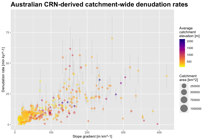
Plot 1. Australian Be-10-derived catchment-averaged denudation rates against average slope gradient
Example 2. Australian sedimentary fluvial OSL ages
For this example we quickly want to display Australian OSL (Optically Stimulated Luminescence) ages on a base map.
library(mapview) # Provides functions for quick visualisation of spatial data
mapviewOptions(fgb = FALSE)
url2 <- parse_url(OCTOPUSdata) # parse URL into list
url2$query <- list(service = "wfs",
                   version = "2.0.0",
                   request = "GetFeature",
                   typename = "be10-denude:sahulsed_fluvial_osl",
                   srsName = "EPSG:900913") # set parameters for url$query

request2 <- build_url(url2) # build request URL from 'url' list
SahulSed.FLV.OSL <- read_sf(request2) # read simple features using 'request' URL. Takes few secs...
SahulSed.FLV.OSL <- st_set_crs(SahulSed.FLV.OSL, 900913) # Set Coordinate Reference System
SahulSed.FLV.OSL = st_transform(SahulSed.FLV.OSL,
        crs = "+proj=longlat +datum=WGS84") # Transform geometry to geographic coordinates, WGS84
mapview(SahulSed.FLV.OSL, xcol = "X_WGS84", ycol = "Y_WGS84",
        zcol = "OSL_AGE", at = seq(0, 350, 50), alpha = .25, # set range (0 to 350 ka) and bins (50 ka)
        alpha.regions = 0.1, legend = TRUE) # Display on map using "mapview" package
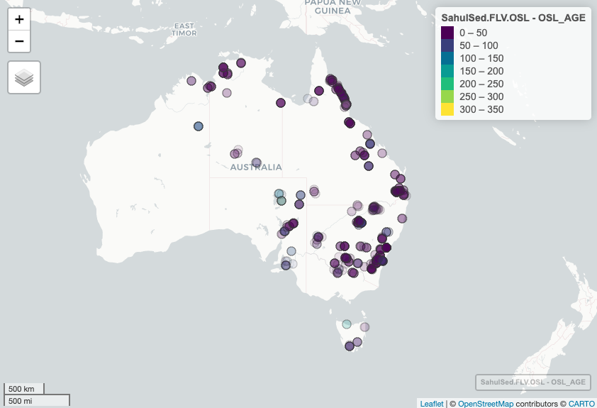
Plot 2. Australian sedimentary fluvial OSL ages
All done!
Tip
Thanks to the very slick ‘Mapview’ 4 functionality, points of the original output map are mouse-over sensitive and can be queried in depth by clicking. Further, the map is scalable and you can choose between a decent selection of base map layers. Try it yourself in R or have a look at a fully functional copy of the above script on RPubs!
Web interface
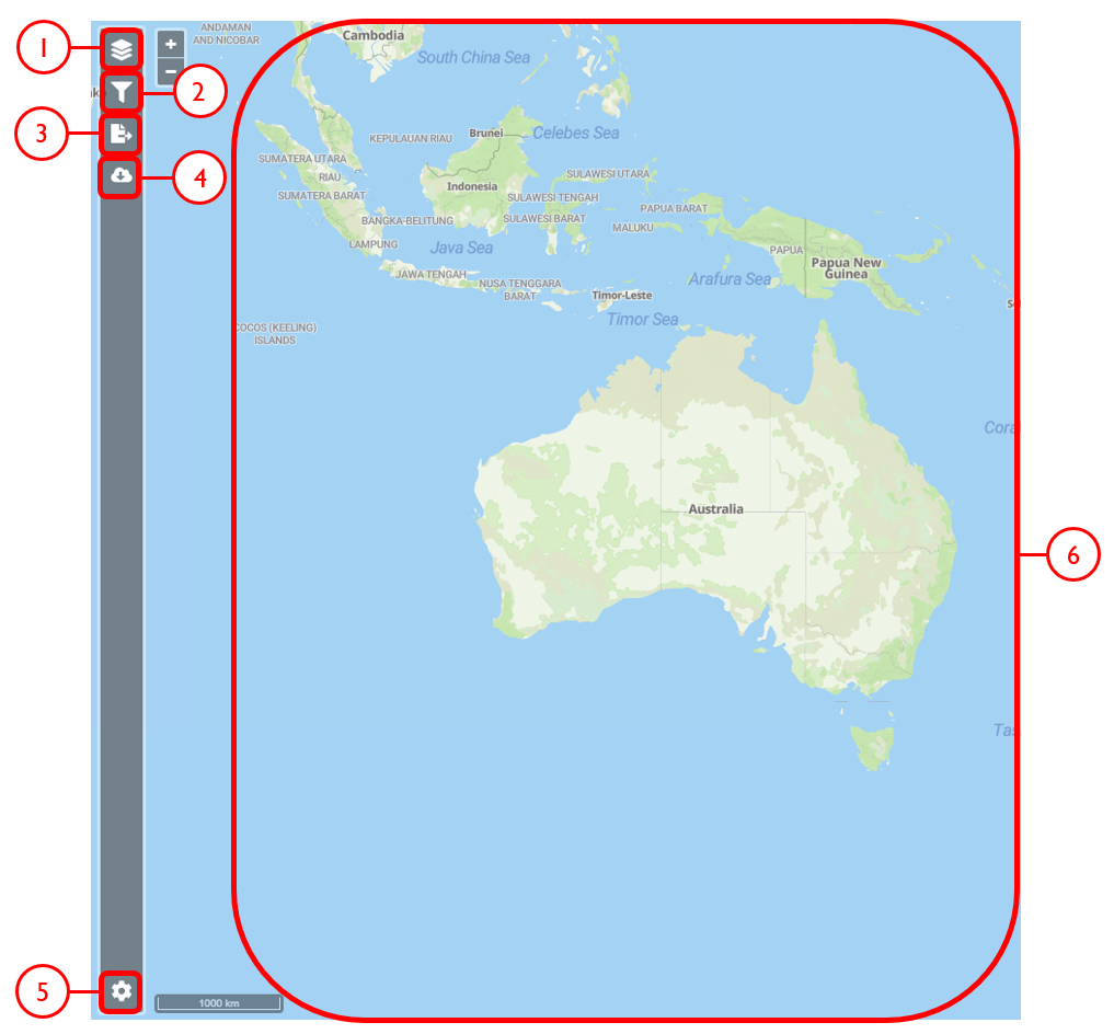
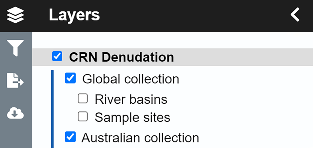
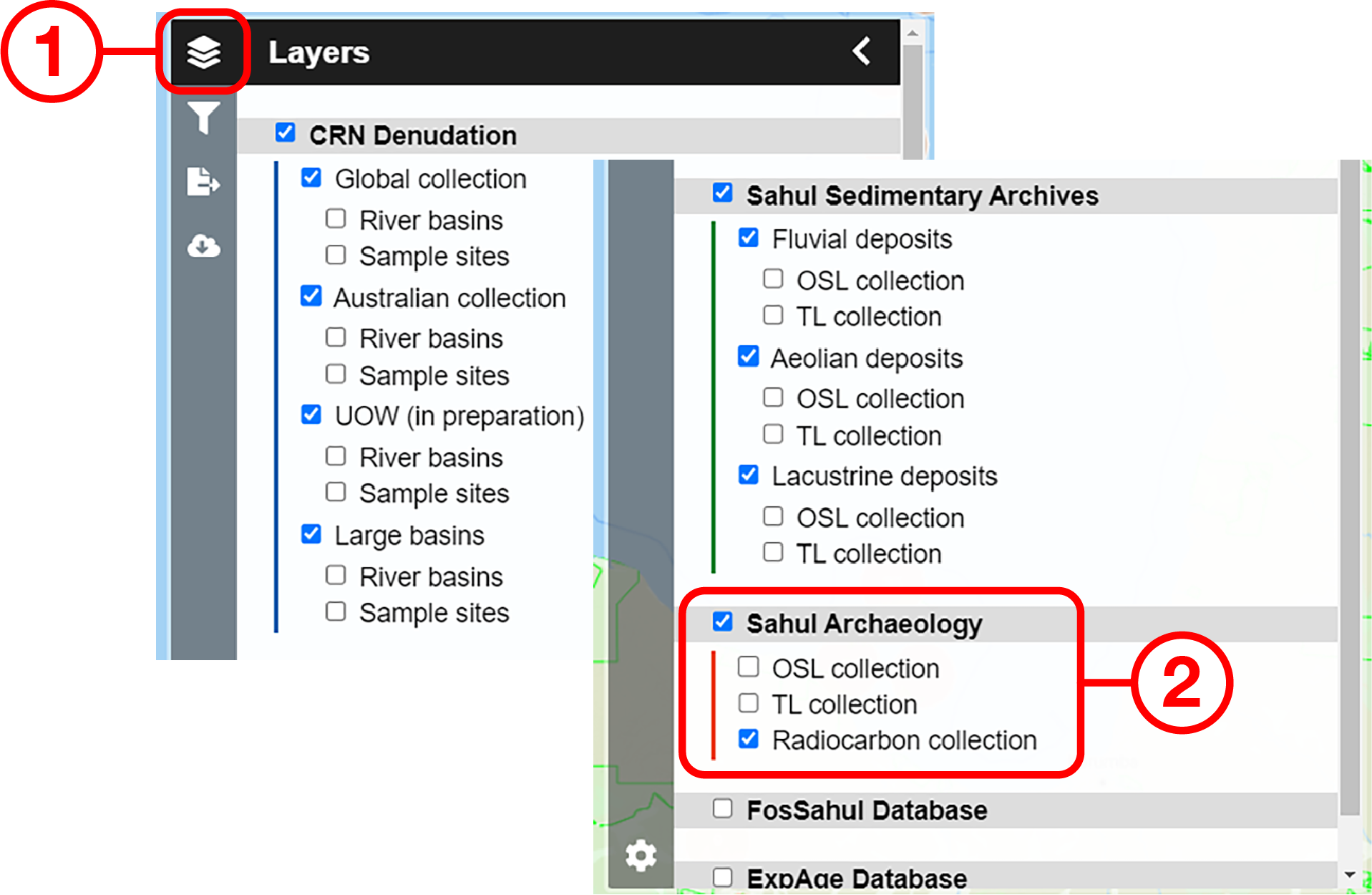
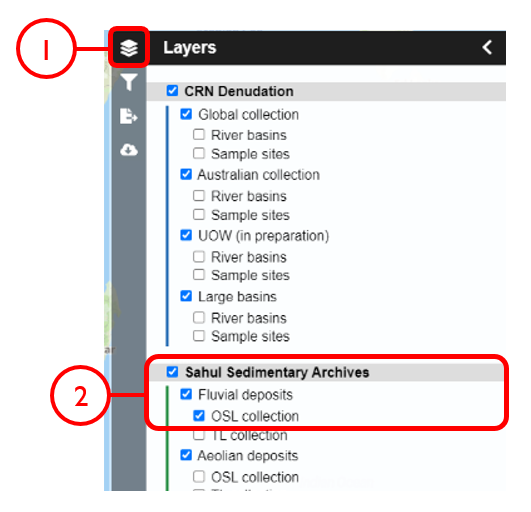
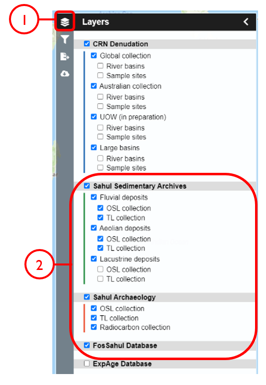
Layers menu
The Layers menu allows you to select data to display, organized by collection. Select tick boxes to view data on the display map.
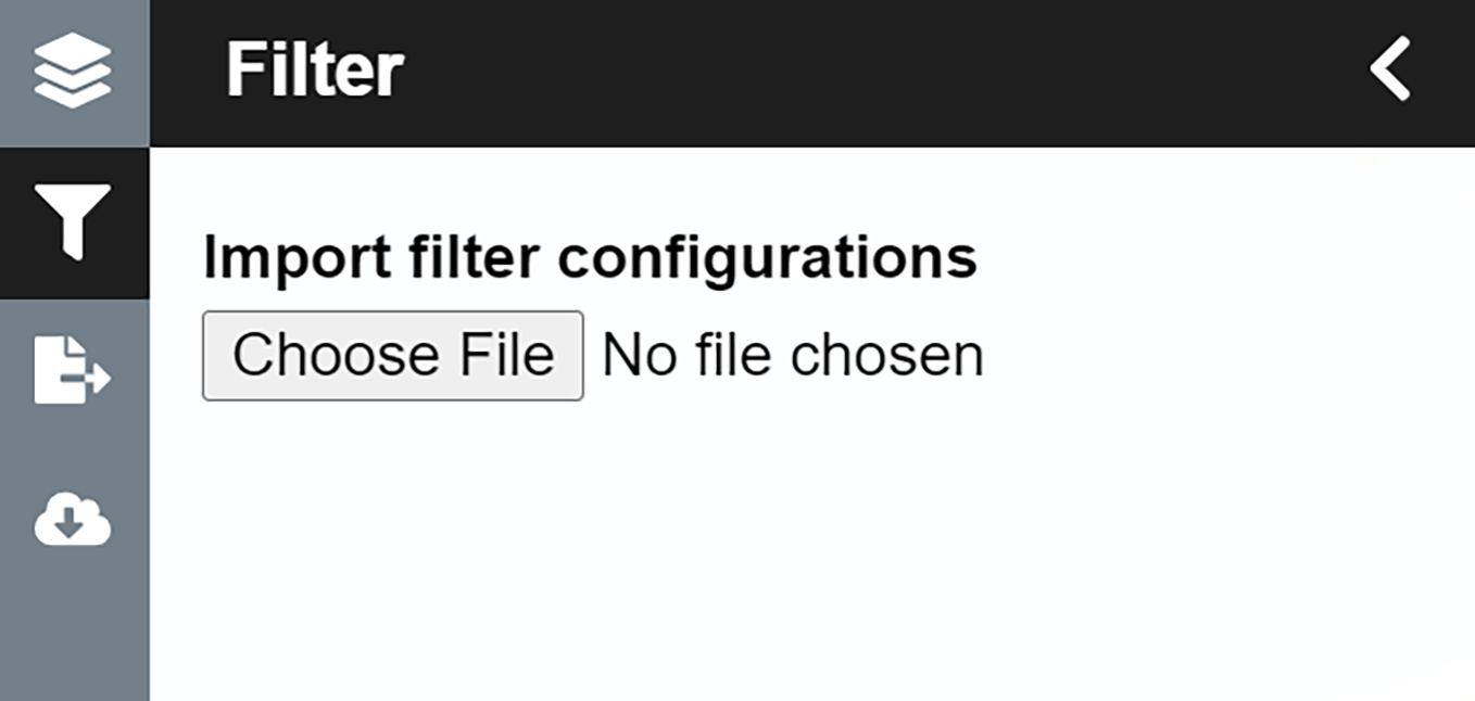
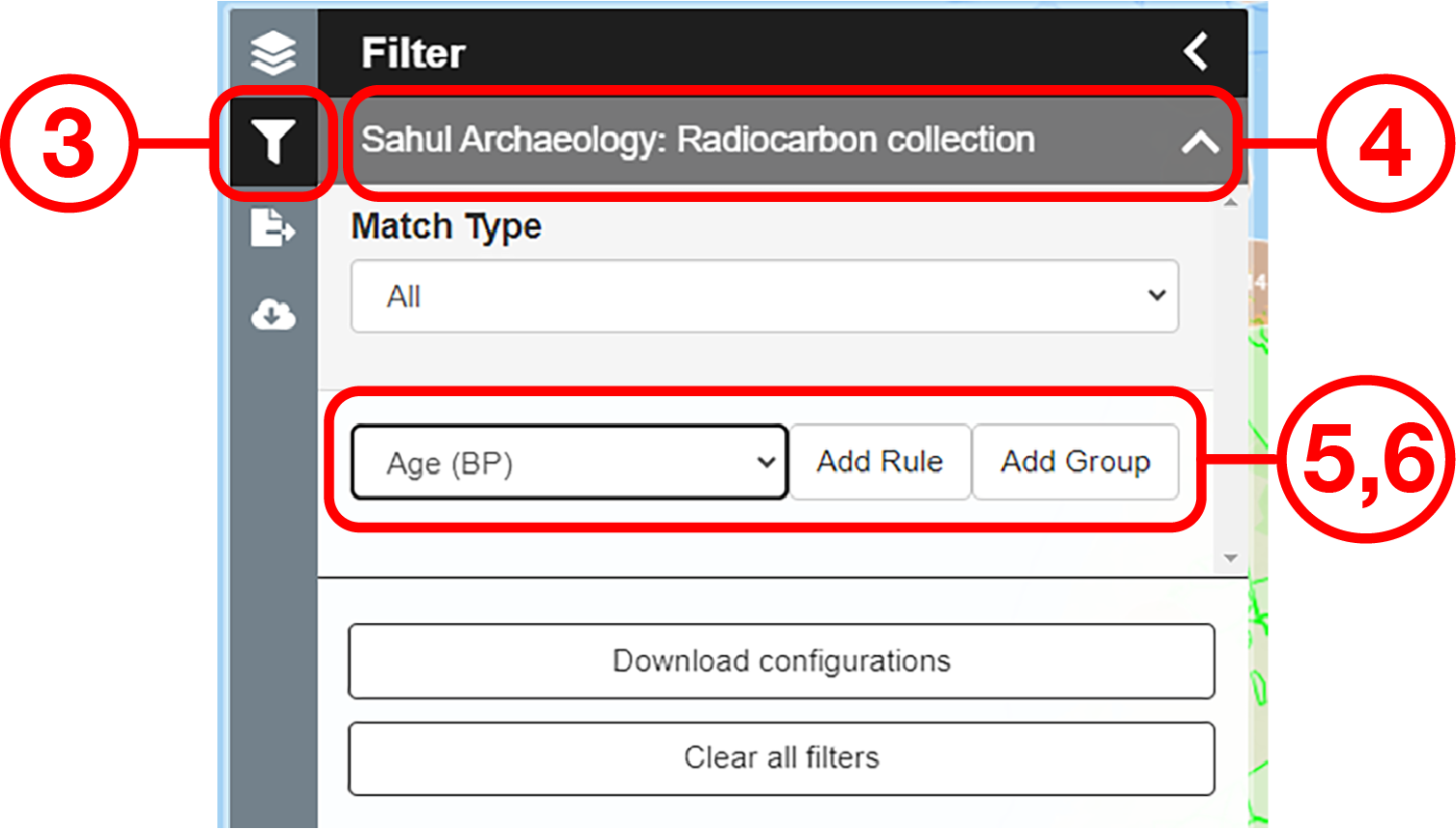
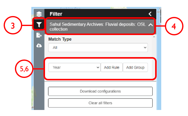
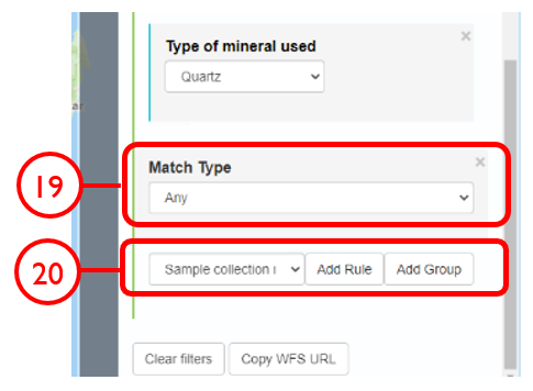
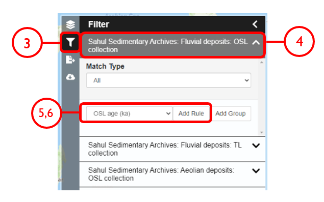
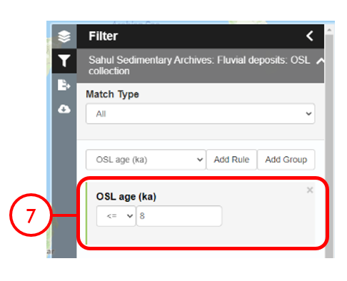
Filter menu
The Filter menu allows you to apply filters to data. You must select at least one dataset to view before you can apply filters, and filters are applied to each data collection individually. In the Filter menu, you can download your filter configuration as a .JSON file and import them.
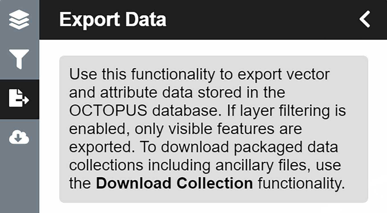
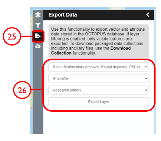
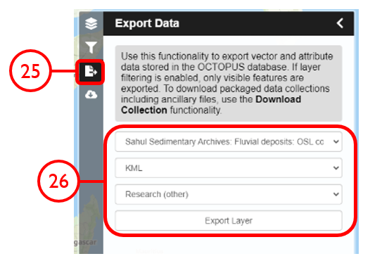
Export Data menu
The Export Data menu allows you to download data, unfiltered or filtered by any rules applied in the Filter menu to that dataset. Data may be exported in the following formats: Geography Markup Language (GML) version 2 and 3, ESRI Shapefile, JavaScript Object Notation (JSON), Google Earth KML and KMZ. You will be prompted to provide an intended use of data prior to download.
Attention
Exported data in the KML and KMZ formats are geographically restricted to the region displayed on screen at the time of export. Zoom in or out prior to export to capture your region of interest. All other export formats include the complete geographic extent of selected data.
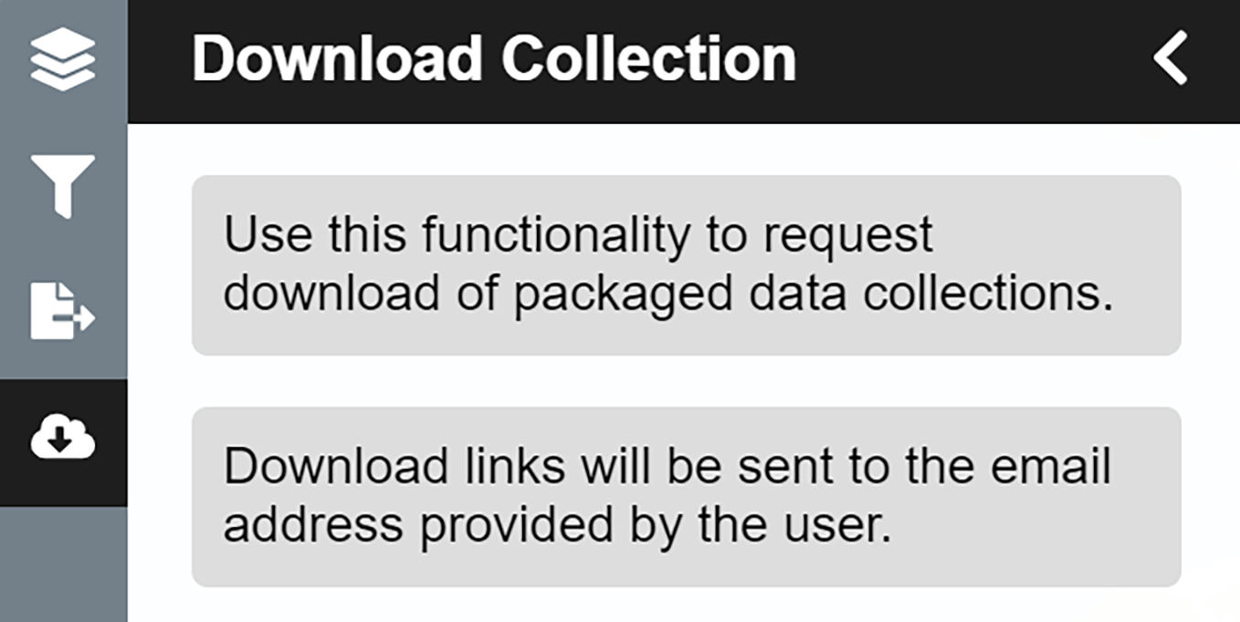
Download Collection menu
The Download Collection menu allows you to request a download of packaged data from the CRN collection. One or more sub-collections from the CRN collection must first be selected in the Layers menu. Hold Ctrl (or cmd on Mac) while clicking and dragging to select a region of interest. You will be prompted within the Download Collection menu to provide a name, email address and intended use of data, and tick boxes for data within your selected region.
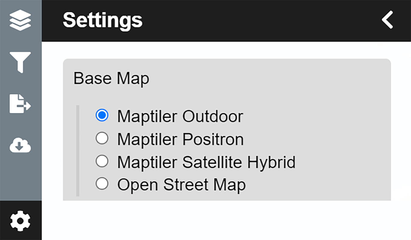
Settings menu
The Settings menu allows you to change the displayed base map, enable case-sensitivity for filters, and control clustering of data.
Data Display menu
Collection data are displayed on a map (see the Settings menu to change base maps) and default to displaying in clusters. Data circles are colour-coded by collection (e.g. Sahul Archaeology: Radiocarbon collection is orange) and show numbers indicating the count of age determinations represented by that circle. The size of circle clusters is also scaled by the number of age determinations it represents. Clicking on a data circle creates a pop-up containing a subset of summary information about the age determinations it represents. Clicking once anywhere in the window outside of the pop-up will close it.
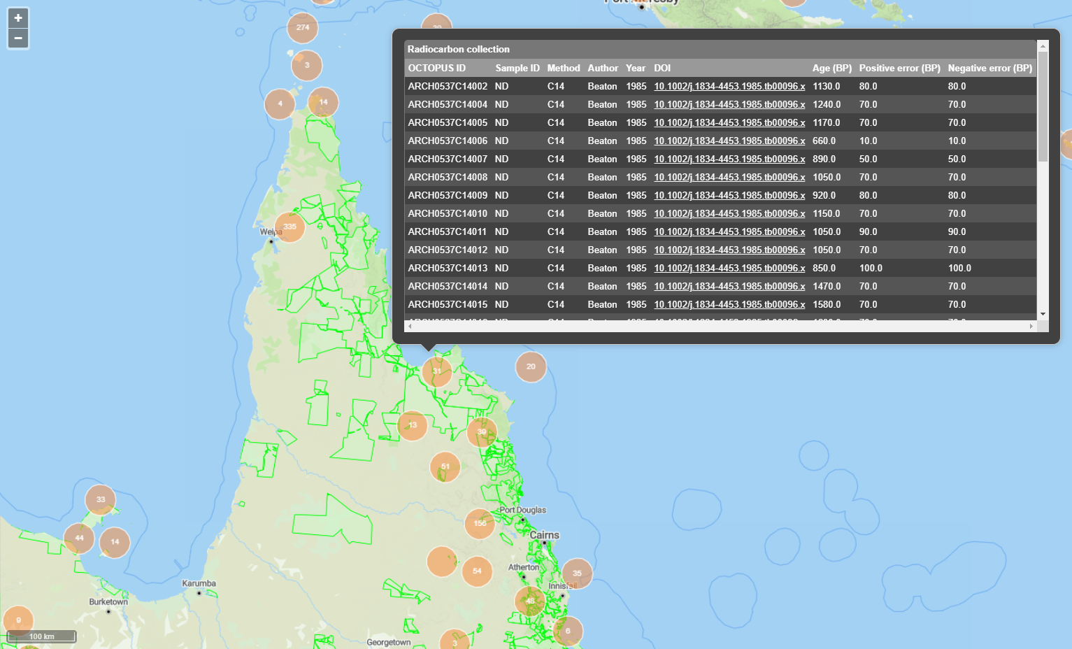
Note
OCTOPUS web interface does not display full data records. To download full data, use the Export Data menu.
Note
SahulArch and FosSahul data points are randomly obfuscated within 25km.
Example use cases
Use case #1
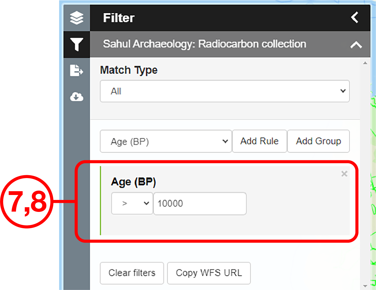
In this example, we will prepare a map of Australian archaeological radiocarbon ages >10,000 BP with a monochrome map and no data point clustering.

Use case #2
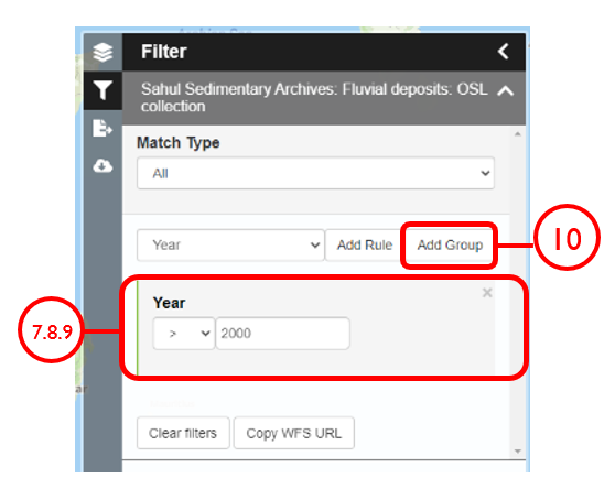
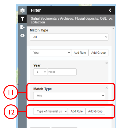
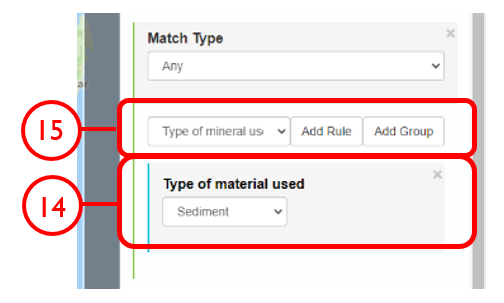
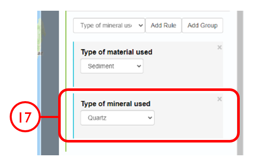
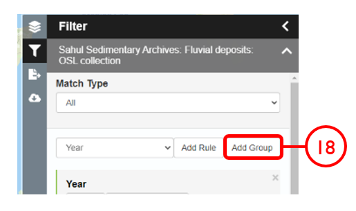
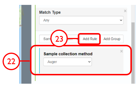
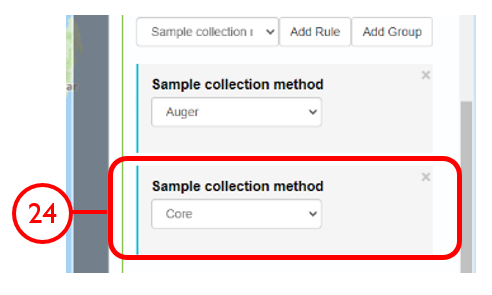
In this example, we will generate a Shapefile of Australian fluvial OSL dates from publications newer than the year 2000, derived from sediments or dating quartz, collected by core or by auger.
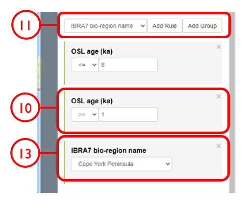
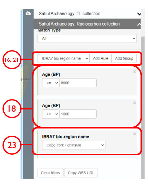
Use case #3
In this example, we will generate KML files of archaeological, fossil, and sediment age determinations from Cape York Peninsula (IBRA bioregion 5) between 1000 and 8000 years old.
Footnotes